Radial distributions
The partial radial distribution g(r) is the pair histogram divided by the ideal gas at the same density. For ice the first peak sits on the oxygen-oxygen contact, near 2.75 angstrom.
The in-plane histogram is the same idea after the coordinates are projected onto a plane. It is the distribution you read for a sheet. A sheet with no thickness at all makes the normaliser undefined, so the monolayer file carries a 0.15 angstrom corrugation. Bulk ice Ih has a well-defined three-dimensional g(r) and a well-defined projection.
# example
import tempfile
from pathlib import Path

import numpy as np
import pydseams as ds
from dseams.userframe import read

from examples.render import IC, IH, panel, save

bulk = ds.read("examples/inputs/ice1h.lammpstrj", atom_type=1)
radius, value = bulk.rdf(1, 1, cutoff=6.0, binwidth=0.1)
radius = np.asarray(radius)
value = np.asarray(value)
peak = int(np.argmax(value))
assert abs(float(radius[peak]) - 2.75) < 1e-6
print("3D peak", float(radius[peak]), float(value[peak]))

sheet = read("examples/inputs/monolayer.lammpstrj", atom_type=1)
r2, g2 = sheet.rdf_2d(tempfile.mkdtemp(), cutoff=8.0, binwidth=0.1)
r2 = np.asarray(r2)
g2 = np.asarray(g2, dtype=float)
assert np.isfinite(g2).all()
peak2 = int(np.argmax(g2))
assert abs(float(r2[peak2]) - 2.75) < 0.2
print("2D peak", float(r2[peak2]), float(g2[peak2]))

chart, ax = panel()
ax.plot(radius, value, color=IH, label="ice Ih, 3D")
ax.set_xlabel("r (A)")
ax.set_ylabel("g(r)")
ax.set_title("Oxygen-oxygen RDF")
ax.legend()
save(chart, Path("docs/images/figures/rdf.png"))

chart, ax = panel()
ax.plot(r2, g2, color=IC)
ax.set_xlabel("r (A)")
ax.set_ylabel("in-plane g(r)")
ax.set_title("Square sheet")
save(chart, Path("docs/images/figures/rdf2d.png"))
# example
using Dseams

sys = System()
seams_system_read(sys, "examples/inputs/ice1h.lammpstrj", 1, 1)
radius, value, volume = seams_rdf(sys; rmax=6.0, bins=60)
peak = argmax(value)
@assert abs(radius[peak] - 2.75) < 1e-6
@assert volume > 0
println(radius[peak], " ", value[peak])
// example
fn main() {
    let mut system = seams::System::new().expect("system");
    system
        .read("examples/inputs/ice1h.lammpstrj", 1, 1)
        .expect("read");
    let g = system
        .rdf(&seams::DistributionOptions {
            rmax: 6.0,
            bins: 60,
            type_i: 1,
            type_j: 1,
        })
        .expect("rdf");
    let peak = g
        .g
        .iter()
        .enumerate()
        .max_by(|a, b| a.1.partial_cmp(b.1).unwrap())
        .unwrap();
    assert!((g.radius[peak.0] - 2.75).abs() < 1e-6);
    println!("peak {} at {}", peak.1, g.radius[peak.0]);
}
# example
set -euo pipefail
seams rdf examples/inputs/ice1h.lammpstrj --pair-types 1,1 --cutoff 6 --bins 60 | tee /tmp/rdf.txt
grep -q "2.75" /tmp/rdf.txt
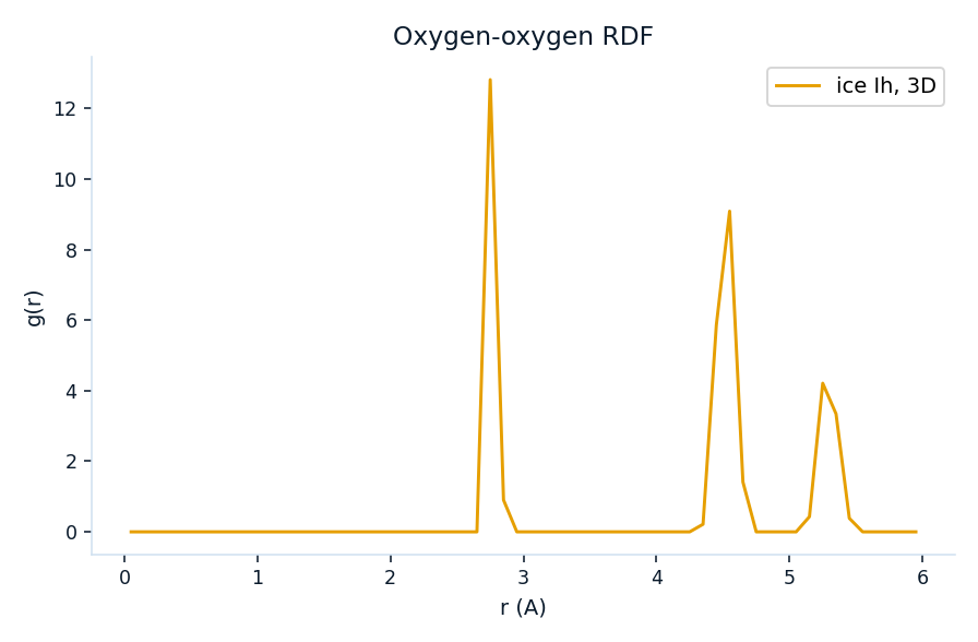
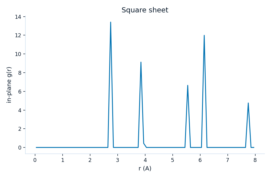
Both histograms peak on the nearest oxygen-oxygen distance. The three-dimensional curve is the bulk crystal. The in-plane curve is the sheet from Monolayer rings. seams rdf is the three-dimensional function. The in-plane writer is the library call in the Python block.